VBA: OLS and SSE

This is a part of our class exercise. Also can be seen in the OLS and SSE excel file. The problem involved:

•  Getting the results of the regression and find the regression estimate per row and compare with the actual, 
• Computing for the error and the squared error
• Displaying the results of regression and the sum of errors in a new worksheet
• Creating a form for that,
• And running the regression program dynamically

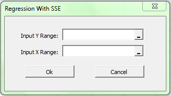
I reused and revised the code in the post Autoregression in functions, in particular the  Function OLS() to regress. In addition, I made up a form getting the data dynamically. Although test for errors were not included.

Functions and Subs

• xM(x1) - Function that creates the x matrix
• CommandButton1_Click() -serves as the test button or the Ok button. or also known as my input - output button because it determines what is your input and creates the output.
• CommandButton2_Click() - the cancel button
• OLS(y, x) - the revised OLS function. Its output are the betas
• SSE(y, x) - solves for the SSE of the regressed y,x

Learning

I spent almost half of the class figuring out why the error mmult property cant run keeps popping up. and after a few hours I found out where I got it wrong. The logic of the code is correct but the parameters of the inputs are wrong. So lesson of the day is: Kung tama ang logic, at mali naman sa pinag gamitan. Mali pa rin yun. It works in real life.

The Form

Simple right :)

The Code

Private Sub CommandButton1_Click()
    y = Range(RefEdit1.Text)
    x1 = Range(RefEdit2.Text)
    
    'creating x matrix
    x = xM(x1)
    
    'regress
    param = OLS(y, x)
    
    'output Sheet
    Sheets.Add
    Range("A1") = "Solution Matrix"
    Range("A" & 2) = "Constant"
    For i = 2 To UBound(param)
        Range("A" & 1 + i) = "x" & i - 1
    Next i
    Range("B2").Select
    ActiveCell.Range(Cells(1, 1), Cells(UBound(param), 1)) = param
    Range("D1") = "Sum of Squared Errors"
    Range("D2") = SSE(y, x)
    
    Unload Me
End Sub

Private Sub CommandButton2_Click()
    Unload Me
End Sub

Private Function xM(x1)
    'adding ones to for coefficients in x matrix
    x = Range(Cells(1, 1), Cells(UBound(x1), UBound(x1, 2) + 1))
    For j = 1 To UBound(x, 2)
        For i = 1 To UBound(x)
            If j = 1 Then
                x(i, j) = 1
            Else
                x(i, j) = x1(i, j - 1)
            End If
        Next i
    Next j
    
    xM = x
End Function
    
Private Function OLS(y, x)
 'regression, getting betas and coefficient
 'given the matrix y and x
    
    xtrans = Application.WorksheetFunction.Transpose(x)
    xtx = Application.WorksheetFunction.MMult(xtrans, x)
    xtxinv = Application.WorksheetFunction.MInverse(xtx)
    xtxinvxt = Application.WorksheetFunction.MMult(xtxinv, xtrans)
    bsol = Application.WorksheetFunction.MMult(xtxinvxt, y)
    OLS = bsol
    
End Function

Private Function SSE(y, x)
    'sum of squared errors
    
    param = OLS(y, x)
    
    model = Application.WorksheetFunction.MMult(x, param)
    
    SumErrors = 0
    For i = 1 To UBound(x)
        SumErrors = SumErrors + (y(i, 1) - model(i, 1)) ^ 2
    Next i
    
    SSE = SumErrors
End Function

Interest Rate Models

The class groups discussed two of term structure models: The Vacisek Model and the CIR term model.  These models are used to model interest rates.

What about the models:

• equilibrium type of model
• uses the Mean Reversion 
• offer benefits since they are numerically quite simple and easy to solve with computers
• very helpful in finding the important factors. 
• interesting and widely tested empirically since they offer closed form solutions of their conditional and steady state density functions.
• possible to get negative interest rates

Given the following:

• $\Delta t = T-t$ 
• $a$ as the speed of mean reversion
• $\mu$ as the long run average rate
• $r$ as the current state
• $\sigma$ as the volatility

We can get the models:

CIR Model:
\[ P(t,T) = A(T-t)e^{-B(T-t)r}\]
where: \[ A(T-t) = \left [   \frac{2 \gamma e^{(a+ \gamma)(T-t)/2}} {(\gamma +a)(e^{\gamma (T-t)}-1} \right ]^{2ab/ \sigma^2} \]
and
\[ B(T-t) = \frac {2(e^{\gamma (T-t)}-1)}{(\gamma+ a)(e^{\gamma (T-t)}-1)+2 \gamma}\]


Vacisek Model:
\[ P(t,T) = A(T-t)e^{-B(T-t)r}\]

where: \[ A(T-t) = \text{exp} \left [ \frac{ ( B(T-t) - T+t ) (a^2b-\sigma^2/2)}{a^2} -\frac{\sigma^2 B(T-t)^2}{4a}\right ] \]
and
\[ B(T-t) = \frac {1-e^{-a(T-t)}}{a}\]

Comparing these two models, they have the same process only that the parameters $ A(T-t)$ and  $B(T-t)$ are different.


Sources: 

• Hull book
• Groups ppt. They simplified the process.

Monte Carlo Option Pricing

Our group reported on Monte Carlo Option Pricing:

Monte carlo option pricing final v3 from naojan

Notes:

Monte Carlo

• important is how to generate the random distribution.
• Do not rely on this as a black box solution..
• We can look at the historical data.
• We can do this as a project – straight forward models from hull or wilmott to generate the price setting model..to value our payoff.

Slide 3 - The Entire slides focused on Option Pricing. But for Portfolio Statistics we have 3 important concepts:

• Find an algorithm for how the most basic investments evolve randomly. 
• Equities: 
• often the lognormal random walk
• can be represented on a spreadsheet or in code as how a stock price changes from one period to the next by adding on a random return. 
• Fixed-income
• BGM model in modeling how interest rates of various maturities evolve
• Credit 
• A model that models the random bankruptcy of a company. 
• Can represent any interrelationships between investments  which can achieved through correlations.
• Understand the derivatives theory for after performing simulations of the basic investments, there is a need to have models for more complicated contracts that depend on them such as options/derivatives/contingent claims. 
• May be able to use the results in the simulation of thousands future scenarios to examine portfolio statistics 
• Ie. how classical Value at Risk can be estimated

Slide 4

Risk-neutrality assumption – We make the assumption that investors are risk neutral, i.e., investors do not increase the expected return they require from an investment to compensate for increased risk.

Cox and Ross (1976) have shown that the assumption of risk neutrality can be used to obtain solutions of option valuation problems.’ This implies that the expected return on the underlying asset is the risk-free rate and that the discount rate used for the expected payoff on an option  is the risk-free rate.

Slide 6 - Stages from Watsham book and the original Boyle paper

Slide 7 - 14 - Option pricing_monte carlo example.xls

Slide 15 -Example from Wilmott: 

Its difference from watsham is that the watsham example creates random variables with empirical data's probability distribution. Wilmotts random variables are with uniform probability distribution.

***Note: have to understand the "Antithetic and QuasiRandom.xls"

VBA: Bond Valuation II

In our class discussion, the prof taught me a different way of coding using the record macro and worksheets.

• Made me think it will be helpful in creating excel sheet forms and output data.
• Discovered ActiveCell.Offset(r,c)

Here's the code:


Sub Macro3()

For i = 1 To 108

Application.ScreenUpdating = False

Sheets("DATA Process").Select
Range("A1").Select

'dito ka lng nagloop and it works for all
ActiveCell.Offset(i, 0).Range("A1:E1").Select
Selection.Copy

Sheets("Scratch").Select
Range("A2").Select
Selection.PasteSpecial Paste:=xlPasteValues, Operation:=xlNone, SkipBlanks _
        :=False, Transpose:=False

Range("F15").Select
Selection.Copy

Sheets("DATA Process").Select
ActiveCell.Offset(0, 6).Range("A1").Select
Selection.PasteSpecial Paste:=xlPasteValues, Operation:=xlNone, SkipBlanks _
        :=False, Transpose:=False

Next i

End Sub

VBA: Short Lecture Notes

Steps/Pointers for doing your code:

• Outline what you need to do in little modules.
• For each major procedure make an outline
• Try out the procedures on the spreadsheet 
•  Automate using the macro 
• Clean up the macro and do your editing. (Doing back engineering)
• Put your procedures together
•   Put your favourite codes together
• Stress test your code
• When in doubt, Use Help.

Some Clarifications

• Procedure: This is a basic set of codes that gets executed: Sub and End sub
•  Functions: creates a dynamic output: Function and End Function
• Modules: see all of your code

Variables: Common Data Type

• It must really be defined.
• Common Data Types
• Integers
• Long
• Single
• Double
• Decimal
• Date
• Object
• String - text
• Variant – any kind
• String x integer = error, so define the variables beforehand
• It entails dimensioning
• Data type Summary on VBA Help for more information

Declaring Variables 

• Code: Dim a as Integer, b as integer
• Declaring arrays
• Dim histdata(1 to 100) as double - it has 100 items
• Dim matrix(100,100) – it has 101 x 101 items

Looping

• For next
• For each next -
• Do while Loop – continue running until true
• Do until 
• Do – can endlessly run

If then Statements

     If a<b 

       Variable = 0

     Else
       Variable = 1
     End if
  

 Go to statement

• Changes the flow of the procedure
• BEST used for error trapping
• Abruptly change the code..
• Example: if variable = 1000, go to 170 (which is a statement outside the loop)
• Best used for error trapping

Case Constructions

• Works like if then statement, very handy for multiple cases

      Select case statement
         Case is <.5
            Procedure for case
         Case else
            Procedure

      End Select
                           
Visual programming - Forms

•  Codes are built around Forms
• In forms event are activated
• Left mouse click
• Click
• Enter range of values
• Working around the form: example: where you can capture the data at outputs the regression
• Form contain objects such as references, command button etc.
• Build form on arrays

Making Add-ins in excel

VBA: Intro to Userforms

Tips and Pointers:

1. Creating a new form: On the Insert Menu, Click Userform.
2. You can change name or label of userform in its Properties section. 
3. A form that choose a matrix or data from excel sheet: RefEdit in Toolbox. If there is no RefEdit, Right click on ToolBox--> Additional Controls --> Check refedit.ctrl --> Ok.
4. Double click on the object itself to view Code. OR On the Project Box, Forms folder, Right click on the form and select View Code.
5. To get the range in refedit: NewName = Range(RefeditName.Text)
6. To run the userform:  FormName.show
7. To end the userform: Unload Me

Additional New Codes:

1. Sheets.Add => adding new Sheets
2. Range("A5").Activate => activating the range

Example Process:

Given two matrices of unknown dimensions, we want to multiply them. 

1. Using the Button "Multiply!" in Excel, it opens up the Userform for Matrix Multiplication.

2. Select the two Matrix to multiply.

3. Click Ok, and then the answers will appear in a new sheet.

4. If wrong dimensions, a msgBox will appear.

5.Clicking the Cancel Button will end the Userform.

Code: userform mmult.xlsm

Sub Macro1()

    'For Button Multiply!

    MatrixMult.Show

End Sub

Private Sub CancelBut1_Click()

    Unload Me

End Sub

Private Sub OkBut1_Click()

    MatrixA = Range(mA.Text)

    MatrixB = Range(mB.Text)

    

    'Checker

    If UBound(MatrixA) = UBound(MatrixB) And UBound(MatrixA, 2) = UBound(MatrixB, 2) Then

        'Start of MMult

        r = UBound(MatrixA)

        c = UBound(MatrixA, 2)

    

        Sheets.Add

        ActiveCell.Range("A1").Select

        ActiveCell.Range(Cells(1, 1), Cells(r, c)) = Application.WorksheetFunction.MMult(MatrixA, MatrixB)

    Else

        MsgBox "Wrong dimensions of matrices"

    End If

    

End Sub

VBA: Autoregression

The code calls for the range of the original series, and the number of lags we wanted for the autoregression.  then OLS in matrix form is performed with the output of the betas and coefficient of the model. Again this is not dynamic

And oh..I'm getting the used to adding watches and stops.

Sub regression()

    'calling for fixed range and lag values
    orig = Range("B3:B100")
    lag = 2
    
    r = Range("B3:B100").Rows.Count - lag
    y = Range(Cells(1, 1), Cells(r, 1))
    For i = 1 To r
        y(i, 1) = orig(i + lag, 1)
    Next i
    
    'creating x range
    c = lag + 1
    x = Range(Cells(1, 1), Cells(r, c))
    
    'individual, not dynamic
    'For i1 = 1 To r
    '    x(i1, 1) = 1
    'Next i1
    
    'For i2 = 1 To r
    '    x(i2, 2) = orig(i2 + 1, 1)
    'Next i2
    
    'For i3 = 1 To r
    '    x(i3, 3) = orig(i3 + 0, 1)
    'Next i3
    
    For j = 1 To c
        For i = 1 To r
              x(i, j) = orig(i + c - j, 1)
              If j = 1 Then x(i, j) = 1
        Next i
    Next j
    
    'Range("i7").Select
    'ActiveCell.Range(Cells(1, 1), Cells(r, 1)) = y
    'Range("j7").Select
    'ActiveCell.Range(Cells(1, 1), Cells(r, c)) = x
    
    'regression, getting b solution
    xtrans = Application.WorksheetFunction.Transpose(x)
    xtx = Application.WorksheetFunction.MMult(xtrans, x)
    xtxinv = Application.WorksheetFunction.MInverse(xtx)
    xtxinvxt = Application.WorksheetFunction.MMult(xtxinv, xtrans)
    bsol = Application.WorksheetFunction.MMult(xtxinvxt, y)

    'output in the excel
    Range("H6") = "b="
    Range("I6").Select
    ActiveCell.Range(Cells(1, 1), Cells(c, 1)) = bsol
    
End Sub

Autoregression Sample

Sample Auto regression of Stock returns in Excel

Recall: 
\[AR(2): y_t = b_0+b_1y_{t-1}+b_2y_{t-2}+ \text{error}\]
Process in Excel. (pls see autoregression.xlsm)

1. Since we want an AR(2), we first get the lag1 and lag2 of the original stock return as shown below.

2. From the Data Ribbon, click Data Analysis on the left side of the Ribbon.

3. Choose Regression, then click OK.

4. For the Input Y Range, choose the original series.

5. For the Input X Range, choose the lag series.

6. Remember to only choose the number of observations that both Y and X have. Unfilled Cells are disregarded. That means for the Y series, we chose B5:B100 and for the X series we chose C5:D100.

7. Click OK.

Results and Interpretation:

With 96 observations, the model resulted to an AR(2) with the linear combination of
\[ y_t = 0.00679131-0.0066908y_{t-1}-0.0486791y_{t-2}+ \text{error}\]
However, The F Statistics shows us that the value is greater than alpha of 0.05. It implies that the model does not fit to the data given. Moreover, the Adjusted $R^2=-0.01$ which implies that only -0.1% of the variance was explained.  Furthermore, the betas and the coefficient are not significant as their p-values are greater than alpha of 0.05. These leads us to the analysis that even though we got the model, it is not a good model to begin with. At least we know now how to do regression in Excel. :-)

Time Series Analysis

Trend Line - OLS

•  It has four major assumptions
• line
• normal distribution
• equal variance
• serial correlation (looking at the area of volatility)
• if not linear - transformation should occur. and anything transformed should revert it back to the original.

Autoregression

• regressing data against itself  - lags (for an example of how to in excel, see autoregression.xlsm)
• Sample model: $AR(2): y_t = b_0+b_1y_{t-1}+b_2y_{t-2}+ \text{error}$

Moving Average

• Sample model: $MA(2): y_t = e_0 +a_1e_{t-1}+a_2e_{t-2}$
• the $e$'s are the errors of an internal model.

ARMA

• Combination of both AR and MA Model
• Sample model: $ARMA(2,2): y_t =b_0+b_1y_{t-1}+b_2y_{t-2}+ e_0 +a_1e_{t-1}+a_2e_{t-2}$
• $AR(1):  y_t =b_0+b_1y_{t-1}+\text{error} $
• $b_1 <1$ - no problem. It stays stationary even if there are shocks.
• $b_1=1$ - shocks has permanent effect in the time series model.
• $b_1>1$ - not stationary. It explodes or decays.
• Covariance stationary
• mean is constant over time
• variance and covariance is constant over time
• $MA(1): y_t = e_0 +a_1e_{t-1}$
• the errors are artifacts of another model and its always brand new.
• Box-Jenkins
• AR
• ACF - decay to 0
• PACF -drops to 0
• MA
• ACF - drops to 0
• ACF - decay to 0
• Parsimony - important, how good is the forecast?
• AIC and BIC - choosing the model with the lowest value
• Random walk
• Model: $y_t = y_{t-1} + e$
• if the first differences is a white noise process.

Integrated Model

• If we difference it twice, we must go back twice after.
• ARIMA(p, d, q) model - AR(p), integration at d, MA(q)

Business Modelling

• MA - Kathang isip lamang because of the errors
• AR - is based on observable values
• Rule of thumb - 50 observations

Random walk with Drift

• An AR model:  $AR(2): y_t = b_0+b_1y_{t-1}+b_2y_{t-2}+ \text{error}$
• it is a random walk with trend

Mean Reversion

• MPT Application: Variance = $w^T \sigma w$ (sensitivity analysis on variancesensitivity.xlsx)
• must be homoscedastic
• not work on negatives

GARCH

• Conditional Heteroscedasticity applies
• Model:  $GARCH(1,1): h_t = \alpha_0+\alpha_1r_{t-1}^2+\beta_1h_{t-1}$

EWMA

CRR Tree

Since we are assigned to report on the CRR tree, our group made a powerpoint presentation on this. It includes the basics of a CRR tree.

Crr presentation from naojan

Notes: CRR presentation.pptx, CRRBOPMv2.xlsx

Jarrow-Rudd Tree (JR) tree is assumes 50% probability in the u and d. CRR don't.

Slide 6 

Step 1. Binomial model acts similarly to the asset that exists in a risk neutral world.

\[ pu+qd = e^{i * \Delta t} = r\]

where

\[\begin{split}
\Delta t &= \frac{t}{n} \\
t &= \text{term of the option} \\
n &= \text{number of periods}
\end{split}\]

Its variance: 

 \[ pu^2 + qd^2 – e^{(i* \Delta t)^2} = \sigma^2 \Delta t \]

Slide 9 - Notice that the lattice is symmetrical, that is due to the assumption that d=1/u (ud=1). Thus , it is easier to program since it involves fewer steps.

References:

• Cox, J.C., Ross S.A, Rubinstein, M., Option Pricing : A Simplified Approach. (1979). Published in Journal of Finance and Economics
• Watsham, Terry J., and Parramore, Keith. Quantitative Methods in Finance. (1997)
• http://investexcel.net/736/binomial-option-pricing-excel/
• http://www.sitmo.com/article/binomial-and-trinomial-trees/
• http://en.wikipedia.org/wiki/Binomial_options_pricing_model
• http://sfb649.wiwi.hu-berlin.de/fedc_homepage/xplore/tutorials/xlghtmlnode63.html#bin-fig2
• http://www.terry.uga.edu/~mayhew/Old/chapter9.pdf
• Other books:
• Hull book 
• Paul Wilmott
• Advance Modelling in Finance Using Excel and VBA

PCA and FA I

Principal Components Analysis 

    - answers the question " what are the major contributors to the overall variability?"
    - so we look at the "dependent" variables and analyze them

Sample Application:

• Age Groups as variable - who among the age group contributes more. 
• What moves the bond return the most? 
• First, we make a lot of guesses on the x's variables such as:
• tenor
• coupon rate
• yield
• credit rating
• duration
• demand for the bond
• inflation expectation
• supply
• money supply
• political stability
• GDP expectation
• Next, we eliminate the some of the variables based on redundancy, data, etc.
• credit ratings are all risk free (means 0 variance), so we eliminate it.
• demand and supply are related. It can be considered as one. 
• political stability is not measurable.
• Then, we determine the data for the other variables as they are measurable
• tenor
• coupon rate
• yield
• duration
• demand and supply for the bond - bid ask spread
• inflation expectation - BSP futures curve or consensus estimate for GDP
• money supply - entry growth BSP
• GDP expectation 
• we now can apply PCA to the variables

Applying PCA to the x variables

• From the variance-covariance matrix, we get the correlation matrix. It is so because the data needs to be normalized first and we are able to achieve it by dividing the data by the standard deviation. And correlation matrix is the standardized form of the variance-covariance matrix.
• Then get eigenvectors and the eigenvalues.
• Eigenvectors - produce the matrix of linear combinations 
• Eigenvalues - its total sum is the total number of variables in the standardized matrix
• each eigenvector (linear combination) has its own eigenvalue 
• Interpretation of the eigenvectors and the eigenvalues
• divide the each eigenvalue by its sum gives us the proportion that eigenvector accounts to the total variance. The higher the proportion the more significant its contribution to the total variability. 
• Some says that getting eigenvalues greater than 1 are the ones that are significant. So we disregard the ones that are less than one since they are not significant.
• As application in portfolio management, this gives the portfolio manager the opportunity to adjust the weights of the portfolio components so as to reduce the element of risk.

  Factor Analysis

• main focus: summarization and data reduction
• Given the variables, it answers the question "What drives the variables?"
• this analysis is an ends by itself  or can be a part of a process
• Stock = A Factor1 + B Factor2 + C Factor3, where the factors are the groups.

Example: 

Given stocks 1-10, (in the dummy stocks excel, and quant prof) we apply factor analysis. First we get the correlation matrix from group statistics, and then apply factor analysis with the correlation matrix.

From the unrotated loadings, we determine each group or factor by ranking as shown on the example below.

There are other ways to get the factor analysis. What is important is that we know how to analyze the data given.

This can be one of the individual projects. can also be ANOVA, test of hypothesis, etc.

PCA and FA application - factoranalysis.xlsx

Consider the linear combinations of 3 factors given below. We assumed that there are 3 factors affecting stockA, B and C.

For Problem1, we want to find the weights to invest in stock A,B and C, considering equal returns for the three stocks. For Problem2, we want to find the weights to invest in stock A,B and C, considering only Stock C returns. This is called one factor analysis. For Problem3, we want to find the weights to invest in stock A,B and C, considering only Stock A and half of Stock C returns. The problem is summarized on the table below.

 Solution:

To solve for the weights, we used the "matrix OLS" as a solution.
\[\hat{y} = \hat{x}\hat{b} \to \hat{b} = \hat{x}^{-1}\hat{y}\]

 In this case $\hat{y}$ is our expected returns, $\hat{b}$ is our weights and \hat{x} is the factors affecting the returns.

With problem 1, we applied multi-factor sensitivity as all of the factors and stocks are considered. After solving for the weights, we have to buy 47% of stock A, sell 77% of stock B and buy 145% of Stock C. Also it is found that we have to borrow 15% since the total sum of the weights is 115%.

Problem 2 only considered Stock C. When we do this, one factor sensitivity is used. As a result in finding for the weights, we have to sell 145% and 174% for stocks A and C respectively. (Can we sell what we don't have??) The total sum of the weights are 9% meaning it is not fully allocated.
 

Problem 3 considers a return for Stock A and half of Stock C only. This results to allocating 60%, 130% and -134% to the stocks A, B and C respectively. Total sum of the weights is 55% which pertains to the total allocation.

Sources: ppt class presentations, class lectures and quantprof VBA

LP and Non-LP Issues

Linear Programming

• Mathematical method used for optimization problems
• Main applications are to maximize profits and minimize costs
• Objective function is linear when:
• Optimum always attained at constraint boundaries
• A local optimum is also global optinum
• Other applications
• operational research - solve multi-commodity flow issues and network flow
• strategic games - chess, manufacturing, resource conservation, transportation systems for buses and trains, and military budgeting
• microeconomics
• Assumptions:
• all variables have non-negative values
• A negative value will be written as a function of two non negative values
• ie. If $x = -5$, then we let $x_1 = 0$, $x_2=5$ and assign $x = x_1 - x_2$
• Advantages:
• Works with inequalities with non negative coefficients. As long as the inequalities are changed into standard form
• The simplex algorithm can determine if there is no solution to the problem (if pivot can't be made)
• Algorithm is easy to program in a computer
• Disadvantages:
• The algorithm becomes inefficient if too many variables are used. It may require an exponential number of steps.
• Strict inequalities might not work in LP
• Example: same example as earlier, using x as the first pivot

Non Linear LP

• Objective function is non linear when:
• Optimum may be interior as well as at boundaries of constraint 
• A local optimum is not necessarily the global optinum
• Nonlinearity came from
• multiplication of variables: economies of scale, transaction costs
• quadratic terms: variances, interest rates mean-variance optimization
• nonlinear functions: quantiles in common risk measures
• Approach to nonlinear optimization: iterative method
• Basic Numerical methods: Solving for non linear functions
• Other methods: 
• Steepest Descent Method
• Newton's Method 
• Quasi-Newton Method
• Lagrange multipliers 
• Conjugate Gradient Method
• Penalty Function Method
• In general, optimization problems are unsolvable.
• "It's the user's responsibility to choose an algorithm that is appropriate for the specific applications

Take-aways

• revised way of pivoting starting with $x$ in the simplex method
• What if the constraints are less than the unknown? Will there be a difference in the simplex method?
• Always check on the assumptions coz it might not gonna work because of wrong constraints
• the answer might not be exactly the solution to the problem at hand. We might be creating more problems than the solution of the problems
• Portfolio optimization technique - "robustness"
• The methods are just tools for the user to use. The question is, is the user using the right tools for the problem at hand?

Resources: Class groups ppt.

History of Finance - Review

Based on Statistics, we can't be always at the top. Whatever we do, we influence the market. So we can't all be winners.

• Pre-Markowitz - make money if your an insider.
• Gerald Loeb 
• the battle for investment survival
• put all your eggs into one basket
• John Maynard Keynes
• Psychological Principle
• The Greater Fool theory
• Beauty Contest Analogue 
•  based on perception, we ask the question: what will the judges judge?
• what do you think the others will think?
• even if I bought at a high price, some other fool will buy at a higher price
• Markowtiz 
• Issue before: How to measure returns
• he introduced risk and how to put up a portfolio and maximize returns
• significant is within the utility curve
• Markowitz Paradox - utility curves 
• Asset universe
• Markowitz -diversification as the risk averse technique
• James Tobins
• optimum portfolio
• don't put your eggs into one basket
• reduce risk using the combination of the risk free rate and others
• we can go outside the Markowitz area
• Simplifying calculus - efficient frontiers labours on calculus
• William Sharpe
• Main feature is the stock market itself
• risk that can be diversified away
• CAPM - Eugene Fama uses the term "one factor model" to describe Sharpe's
• Efficient Market
• Prices fluctuate ramdomly
• Eugene Fama - EMH, 1970
• 1974
• Paul Samuelson
• calls for a benchmark
• if can't beat them, join them
• "Market Portfolio"
• Charles Elis
• Mimic the market - as a proxy for the market
• the use of "index funds"
• it manages the portfolio and costs
• it means no more of the excess returns

Trying to figure out: How to deal with your investments by exerting Alpha.

Alpha - need not to look for weights

• Beta - horizontal
• Alpha - y - intercepts ( excess returns)
• To what degree is the market beatable? Can the market be beaten

Hunt for a better mouse trap

• Multi-factor model 
• Macro-economic Factor Model
• GDP+Analysis => asset allocation
• Industry => asset allocation
• Search for Arbitrage opportunities (buy and sell) and convergence trade (put and call options)
• Search for market anomalies (e.g January effect, small cap effect, low P/B ratios)
• Value vs growth Stocks, underlying stocks Not the company itself
• Contrary strategies
• Risk minimizing modeling (VAR)

References: Searching for Alpha by Ben Warwick

Films: Inside Job, Margin Call, Wall Street Never Sleeps, Wall Street, Too Big to Fail 

Averages, Covariance and Correlation

Recall:

These are some of the important group statistics for portfolio optimization.

1. Averages - a $1$ x $n$ matrix whose inputs are the average of each stocks.
2. Covariance Matrix - the vector product of the mean returns transpose and the mean return itself
3. Correlation Matrix  - $ {cov_{ij}} / {\sqrt{cov_{ii}cov_{jj}}} $

Using functions in VBA

Sub cov()
    Dim str As String
    str = Range("D3")
    
    'calling returns
    ret = Range(str)

    'counting columns
    c = UBound(ret, 2)
    
    'Writing Output
    
    Range("B5") = "Averages"
        'writing answer to averages
        Range("B6").Select
        ActiveCell.Range(Cells(1, 1), Cells(1, c)) = AveM(ret) 'it calls for the function Ave and paste it to a

    Range("B8") = "Covariance Matrix"
        'writing answer to covariance
        Range("B9").Select
        ActiveCell.Range(Cells(1, 1), Cells(c, c)) = CovarianceM(ret)
    
    Range("B" & 10 + c) = "Correlation Matrix"
        'writing answer to correlation
        Range("B" & 11 + c).Select
        cv = CovarianceM(ret)
        ActiveCell.Range(Cells(1, 1), Cells(c, c)) = CorrelationM(cv)
End Sub

Function AveM(ret)
    'summing up all values in each stock and then dividing it by the total number of returns
    
    'counting rows and columns
    r = UBound(ret)
    c = UBound(ret, 2)
        
    'creates 1xc array
    a = Range(Cells(1, 1), Cells(1, c))
    
    'summing up all values in row, then divide it by the row
    For j = 1 To c
        s = 0
        For i = 1 To r
            s = ret(i, j) + s
        Next i
        a(1, j) = s / r
    Next j
        'returns a as the average
        AveM = a
End Function

Function CovarianceM(ret)
    'covariance matrix  = (mean returns transpose x mean returns)/(n-1)
    
    'count rows and columns
    r = UBound(ret)
    c = UBound(ret, 2)
    
    'create dummy range for mean returns
    mret = Range(Cells(1, 1), Cells(r, c))
    
    'create dummy range for average and run the function Ave
    a = Range(Cells(1, 1), Cells(1, c))
    a = AveM(ret)
    
    'solving for mean returns
    For i = 1 To r
        For j = 1 To c
            mret(i, j) = ret(i, j) - a(1, j)
        Next j
    Next i
    
    'solving for transpose and the covariance matrix
    trans = Application.WorksheetFunction.Transpose(mret)
    covm = Application.WorksheetFunction.MMult(trans, mret)
    For i = 1 To c
        For j = 1 To c
            covm(i, j) = covm(i, j) / (r - 1)
        Next j
    Next i
    
    'returning the covariance matrix
    CovarianceM = covm
    
End Function

Function CorrelationM(covm)
    'Correlation Matrix cor_ij = cov_ij / [sqrt(cov_ii)*sqrt(cov_jj)]
    
    'count rows only since covm is an nxn matrix
    r = UBound(covm)
    
    'creating dummy range for cor_ij
    cor = Range(Cells(1, 1), Cells(r, r))
    
    'solving for correlation matrix
    For i = 1 To r
        For j = 1 To r
            cor(i, j) = covm(i, j) / (covm(i, i) * covm(j, j)) ^ (1 / 2)
        Next j
    Next i
    
    CorrelationM = cor
End Function

VBA: Matrix Lecture

Sub matrixP()

'putting the to matrix in an array
a = Range("b3:d5")
b = Range("g3:i5")

'applying matrix multiplication
m = Application.WorksheetFunction.MMult(a, b)
Range("b8:d10") = m

'counting rows and columns
r = Range("b3:d5").Rows.Count
c = Range("b3:d5").Columns.Count

'scalar multiplication
'has to define the array first

cvm = Range("B12:d14")
For i = 1 To r
    For j = 1 To c
        cvm(i, j) = m(i, j) / r
    Next j
Next i
Range("B12:d14") = cvm

________________________________________________________

End Sub

Sub Lecture()
'getting the average

'define returns
a = Range("b3:d5")

'define mean adjusted return
MARM = Range("b9:d11")


For j = 1 To 3
    'average
    m = 0
    For i = 1 To 3
        m = m + a(i, j)
    Next i
    ave = m / 3
    Range("a7").Offset(0, j - 1).Value = ave

    'mean returns
    For kount = 1 To 3
        MARM(kount, j) = a(kount, j) - ave
    Next kount
Next j

Range("B9:D11") = MARM


End Sub
________________________________________________________
Sub Macro3()

'diagonals 1-10
For i = 1 To 10
    Range("a1").Offset(i - 1, i - 1).Value = i
Next i


End Sub
________________________________________________________

Sub Macro4()

'row 10x1, 1-10
For i = 1 To 10
    Range("a" & i) = i
Next i

End Sub

VBA: Covariance Matrix 3

applying what we learned in class to the covariance matrix

This code contains:  averages, mean returns, covariance matrix and changing price to returns.

Sub Cov3()

    Dim ws As Worksheet
    Set ws = Sheets.Add
       
    ws.Range("A1") = "Covariance Matrix"

    ws.Range("A3") = "Prices:"
   
    'prices
    p = Worksheets("Sheet1").Range("B2:K100")
   
    'counting rows and columns
    r = Worksheets("Sheet1").Range("B2:K100").Rows.Count
    c = Worksheets("Sheet1").Range("B2:K100").Columns.Count
   
    'pasting price to ws
    ws.Range("A5").Select
    Set ans = ActiveCell.Range(Cells(1, 1), Cells(r, c))
    ans.Value = p
   
    'Returns
    ws.Range("M3") = "Returns"
       
    'rows of return
    r = r - 1
   
    ret = Range("M6:V103")
    For i = 1 To r
        For j = 1 To c
            ret(i, j) = p(i + 1, j) / p(i, j) - 1
        Next j
    Next i
    Range("M6:V103") = ret
   
    'getting the averages and mean returns
    ws.Range("X3") = "Average"
    ws.Range("AI3") = "Mean Returns"
   
    mret = ws.Range("AI6:AR103")
   
    For j = 1 To c
        'average
        s = 0
        For i = 1 To r
            s = s + ret(i, j)
        Next i
        ave = s / r
        Range("X6").Offset(0, j - 1).Value = ave

        'mean returns
        For kount = 1 To r
        mret(kount, j) = ret(kount, j) - ave
        Next kount
    Next j
   
    ws.Range("AI6:AR103") = mret
       
    'getting the covariance matrix
    ws.Range("AT3") = "Covariance"
    trans = Application.WorksheetFunction.Transpose(mret)
    covm = Application.WorksheetFunction.MMult(trans, mret)
    For i = 1 To c
        For j = 1 To c
            covm(i, j) = covm(i, j) / (r - 1)
        Next j
    Next i
   
    Range("AT6").Select
    Set ans = ActiveCell.Range(Cells(1, 1), Cells(c, c))
    ans.Value = covm
   
End Sub

MPT and Asset Allocation

Modern Portfolio Theory

It's a good thing the group reported  Modern Portfolio Theory.

Additional Information:

• In the optimization $\text{min } \sigma = w^T V w $, the inputs in the diagonal of the covariance matrix $V$ are variances.
• It is important to ask the questions: How did they defined the data used? What constitutes returns? It is not that simple and we have to be objective. We must based it on empirical data and past research.
• What is the use of the Tangency Portfolio? Why is CAL included in the efficient frontier graph?     

The edited graph are copied in Wiki.


• Every stock's expected return is determined by its beta with the tangent portfolio
• Tangent portfolio by definition has the highest SR
• MPT shows only one method of diversifying: managing risk and return. IRL, there are other ways such as go in and out of the market. Since, CAL connects the risk free rate to the tangency portfolio. The highlighted portion is the combination of the risk-free rate and the tangent portfolio which is found to be a way to diversify with a lower risk and still be in the efficient frontier. 
• Any of the portfolios in the upper portion of the $y^2$ curve can beat the market.
• SML - because everyone is buying the market, risk is how much is the market exposure. 
• Empirical data and results shows that MPT is just as it is, a theory. No one can really define and measure the "global market". Some even tested the capacity of CAPM and it doesn't work.

Exercises - found in MPT.xlsm for more info

1. Optimization $\text{min } \sigma = w^T V w $ in Excel. 

2. Covariance

Ways of getting covariance:

In class, we got the covariance of two stocks using the long way and the short way. Details are in the excel sheet. It contains 10 stock returns with an n of 99.

• =COVARIANCE.S(array1, array2)
• =COVARIANCE.P(array1, array2)
• =SUM(x-u_x)(y-u_y)/n

Covariance Matrix

It was also analyzed how the covariance came up to be. 

• It is the matrix multiplication of the mean adjusted return transpose by the mean adjusted return then divided the number of returns
• In short: =mmult(MARTranspose, MAR)/N

Somehow, there are some discrepancies on the numbers I computed for the matrix to the QuantProf, the predefined function made my my prof. But it is very small. Later I found out that some defined =mmult(MARTranspose, MAR)/(N-1) to solve for the covariance matrix.

Other references: Quantitative Methods in Finance by Watsham 

Asset Allocation

• Policy Statement should be there in every portfolio.
• Over long periods of time, sizable allocation to equity will improve results.
• Asset allocation determines your return. It is the overall asset allocation that is important.

Other references involve the previous research material used and a ppt presentation made by another group.

Searching for Alpha

Good reference: Searching for Alpha by Ben Warwick

• History of Finance: Review
• Important people that helped in shaping up the Finance world
• We are trying to figure out how to deal with our investments. Are we satisfied with the the allocation? To what degree is the market predictable? 
• Instead of looking for the weights, we look at alpha.
• where alpha is the excess returns, y-intercepts
• beta is the slope.
• Hunt for a better trap
• Multi-factor model 
• Macro-economic Factor Model
• GDP+Analysis => asset allocation
• Industry => asset allocation
• Search for Arbitrage opportunities (buy and sell) and convergence trade (put and call options)
• Search for market anomalies (e.g January effect, small cap effect, low P/B ratios)
• Value vs growth Stocks, underlying stocks Not the company itself
• Contrary strategies
• Risk minimizing modeling (VAR)

References:

Thursday, February 14, 2013