VBA: OLS and SSE

This is a part of our class exercise. Also can be seen in the OLS and SSE excel file. The problem involved:

•  Getting the results of the regression and find the regression estimate per row and compare with the actual, 
• Computing for the error and the squared error
• Displaying the results of regression and the sum of errors in a new worksheet
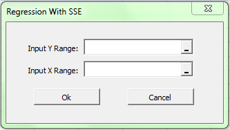
• Creating a form for that,
• And running the regression program dynamically

I reused and revised the code in the post Autoregression in functions, in particular the  Function OLS() to regress. In addition, I made up a form getting the data dynamically. Although test for errors were not included.

Functions and Subs

• xM(x1) - Function that creates the x matrix
• CommandButton1_Click() -serves as the test button or the Ok button. or also known as my input - output button because it determines what is your input and creates the output.
• CommandButton2_Click() - the cancel button
• OLS(y, x) - the revised OLS function. Its output are the betas
• SSE(y, x) - solves for the SSE of the regressed y,x

Learning

I spent almost half of the class figuring out why the error mmult property cant run keeps popping up. and after a few hours I found out where I got it wrong. The logic of the code is correct but the parameters of the inputs are wrong. So lesson of the day is: Kung tama ang logic, at mali naman sa pinag gamitan. Mali pa rin yun. It works in real life.

The Form

Simple right :)

The Code

Private Sub CommandButton1_Click()
    y = Range(RefEdit1.Text)
    x1 = Range(RefEdit2.Text)
    
    'creating x matrix
    x = xM(x1)
    
    'regress
    param = OLS(y, x)
    
    'output Sheet
    Sheets.Add
    Range("A1") = "Solution Matrix"
    Range("A" & 2) = "Constant"
    For i = 2 To UBound(param)
        Range("A" & 1 + i) = "x" & i - 1
    Next i
    Range("B2").Select
    ActiveCell.Range(Cells(1, 1), Cells(UBound(param), 1)) = param
    Range("D1") = "Sum of Squared Errors"
    Range("D2") = SSE(y, x)
    
    Unload Me
End Sub

Private Sub CommandButton2_Click()
    Unload Me
End Sub

Private Function xM(x1)
    'adding ones to for coefficients in x matrix
    x = Range(Cells(1, 1), Cells(UBound(x1), UBound(x1, 2) + 1))
    For j = 1 To UBound(x, 2)
        For i = 1 To UBound(x)
            If j = 1 Then
                x(i, j) = 1
            Else
                x(i, j) = x1(i, j - 1)
            End If
        Next i
    Next j
    
    xM = x
End Function
    
Private Function OLS(y, x)
 'regression, getting betas and coefficient
 'given the matrix y and x
    
    xtrans = Application.WorksheetFunction.Transpose(x)
    xtx = Application.WorksheetFunction.MMult(xtrans, x)
    xtxinv = Application.WorksheetFunction.MInverse(xtx)
    xtxinvxt = Application.WorksheetFunction.MMult(xtxinv, xtrans)
    bsol = Application.WorksheetFunction.MMult(xtxinvxt, y)
    OLS = bsol
    
End Function

Private Function SSE(y, x)
    'sum of squared errors
    
    param = OLS(y, x)
    
    model = Application.WorksheetFunction.MMult(x, param)
    
    SumErrors = 0
    For i = 1 To UBound(x)
        SumErrors = SumErrors + (y(i, 1) - model(i, 1)) ^ 2
    Next i
    
    SSE = SumErrors
End Function

VBA: Autoregression and OLS in functions

The code calls for the range of the original series in one cell and the number of lags to the other cell.  It is assumed that the range of the original series is correct.(Meaning there is no checker for the input of the orig series, but for the lag, there is..) Then we wanted to do autoregression only with this given data.

The AR Function only calls for the original prices and the number of lags we wanted. Inside that function, the y and the x values are created. And then we throw those values to the OLS function where the regression is made.

The function OLS  y and x values as inputs. Since y is now a matrix, we are left with creating the x matrix in such a way that the first columns are 1's. The output would be the betas and coefficient of the model.

It was done as such, so that the OLS(y,x) can function independently. AR(orig,lag) however relies to the OLS function as to how I understood the concept.

The code is written below. It can also be seen in AR functions.xlsm


Sub test()

 'calling for the range and lag values
    Dim ran As String
    ran = Range("J3")
    lag = Range("J4")
    
    If lag < 1 Or lag Like "[A-Z,a-z]" Then MsgBox "Wrong Lag"

    orig = Range(ran)
    
    'output in the excel
    Range("H6") = "b="
    Range("I6").Select
    ActiveCell.Range(Cells(1, 1), Cells(lag + 1, 1)) = AR(orig, lag)

End Sub

Function AR(orig, lag)
    'given original series and number of lag, we apply AR
   
    'creating y values
    r = UBound(orig) - lag
    y = Range(Cells(1, 1), Cells(r, 1))
    For i = 1 To r
        y(i, 1) = orig(i + lag, 1)
    Next i
    
    'creating x values
    x1 = Range(Cells(1, 1), Cells(r, lag))
    
    For j = 1 To lag
        For i = 1 To r
              x1(i, j) = orig(i + lag - j, 1)
        Next i
    Next j

    AR = OLS(y, x1)
    
End Function

Function OLS(y, x1)
 'regression, getting betas and coefficient
 'given values y and x (not the matrix x)

    'adding ones to for coefficients in x matrix
    x = Range(Cells(1, 1), Cells(UBound(x1), UBound(x1, 2) + 1))
    For j = 1 To UBound(x, 2)
        For i = 1 To UBound(x)
            If j = 1 Then
                x(i, j) = 1
            Else
                x(i, j) = x1(i, j - 1)
            End If
        Next i
    Next j
    
    xtrans = Application.WorksheetFunction.Transpose(x)
    xtx = Application.WorksheetFunction.MMult(xtrans, x)
    xtxinv = Application.WorksheetFunction.MInverse(xtx)
    xtxinvxt = Application.WorksheetFunction.MMult(xtxinv, xtrans)
    bsol = Application.WorksheetFunction.MMult(xtxinvxt, y)
    OLS = bsol
    
End Function

VBA: Autoregression

The code calls for the range of the original series, and the number of lags we wanted for the autoregression.  then OLS in matrix form is performed with the output of the betas and coefficient of the model. Again this is not dynamic

And oh..I'm getting the used to adding watches and stops.

Sub regression()

    'calling for fixed range and lag values
    orig = Range("B3:B100")
    lag = 2
    
    r = Range("B3:B100").Rows.Count - lag
    y = Range(Cells(1, 1), Cells(r, 1))
    For i = 1 To r
        y(i, 1) = orig(i + lag, 1)
    Next i
    
    'creating x range
    c = lag + 1
    x = Range(Cells(1, 1), Cells(r, c))
    
    'individual, not dynamic
    'For i1 = 1 To r
    '    x(i1, 1) = 1
    'Next i1
    
    'For i2 = 1 To r
    '    x(i2, 2) = orig(i2 + 1, 1)
    'Next i2
    
    'For i3 = 1 To r
    '    x(i3, 3) = orig(i3 + 0, 1)
    'Next i3
    
    For j = 1 To c
        For i = 1 To r
              x(i, j) = orig(i + c - j, 1)
              If j = 1 Then x(i, j) = 1
        Next i
    Next j
    
    'Range("i7").Select
    'ActiveCell.Range(Cells(1, 1), Cells(r, 1)) = y
    'Range("j7").Select
    'ActiveCell.Range(Cells(1, 1), Cells(r, c)) = x
    
    'regression, getting b solution
    xtrans = Application.WorksheetFunction.Transpose(x)
    xtx = Application.WorksheetFunction.MMult(xtrans, x)
    xtxinv = Application.WorksheetFunction.MInverse(xtx)
    xtxinvxt = Application.WorksheetFunction.MMult(xtxinv, xtrans)
    bsol = Application.WorksheetFunction.MMult(xtxinvxt, y)

    'output in the excel
    Range("H6") = "b="
    Range("I6").Select
    ActiveCell.Range(Cells(1, 1), Cells(c, 1)) = bsol
    
End Sub

Matrices in OLS II

The Technicals

In the book Quantitative Methods in Finance by Watsham and Parramore and in class, it tells us how in empirical data, the series of $x$'s or the matrix with $x$ variables are usually not square, thus not invertible. We just have to work on what was given which are  $\hat{x}$ and  $\hat{y}$.
That's why we have to transform \[ \hat{b} = \hat{x}^{-1}\hat{y} \] into
\[ \hat{b} = (\hat{x}^T \hat{x})^{-1} \hat{x}^T \hat{y}\]
To transform it, identity is used and so is $\hat{x}^T$ as can be seen below.  This is to satisfy my curiosity about the identity.
\[ \begin{array}{rl} b = & x^{-1}y & \\
= & x^{-1}I_n y \\
= & x^{-1}(x x^{-1})^T y \\
= & x^{-1}(x^{-1})^T x^T y \\
= & (x^T x)^{-1} (x^T y)
 \end{array} \]
I looked for other ways to simplify the equation but so far, this is the easiest with the given data.

Application Found

• Regression Analysis (of course) - The measurement of change in one variable (y)  that is the result of changes in other variables (x) . Regression analysis is used frequently in identifying the variables that affect a certain stock's price.
• Hedging or Hedge Ratio (211-212 book)

OLS Macro I

Code lies on matrixOLS.xlsm

Sub olsmaker()
' this solves for regression calling on fixed number of dataset
' Also matrix form is defined by the user.

    'calling for x and y
    x = Range("A105:B114").Value
    y = Range("C105:C114").Value
    
    'solving for b=(xT x)^-1 (xT y)
    xT = Application.WorksheetFunction.Transpose(x)
    xTx = Application.WorksheetFunction.MMult(xT, x)
    xTxinv = Application.WorksheetFunction.MInverse(xTx)
    xTxinvxT = Application.WorksheetFunction.MMult(xTxinv, xT)
    sol = Application.WorksheetFunction.MMult(xTxinvxT, y)

    'returning it back to the sheet
    Range("F106") = "b="
    Range("F107:F108").Value = sol

End Sub

Notes:
1. How do I make it dynamic? Update this program.
2. Review on Matrix and OLS. Work on how did this happened. And is there a way to shorten the form?
 \[ \hat{b} = \hat{x}^{-1}\hat{y} \to \hat{b} = (\hat{x}^T \hat{x})^{-1} \hat{x}^T \hat{y} \]
3. Very interested in programming numerical methods. Add it to the List to program.
4. Read the book: VB for Dummies.

Matrices in OLS

Matrix Multiplication

If $A$ and $B$ is $3$ x $3$ matrix, then $AB$ is also a $3$ x $3$ matrix. However $AB \neq BA$ because matrix multiplication is not commutative.

As an illustration: matrixOLS.xlsm

\[ A =  \begin{bmatrix}
1 & 2 &3 \\
4 & 5 & 6 \\
7 & 8 & 9
\end{bmatrix}
\;\;\;\;\;
B =  \begin{bmatrix}
11 & 12 &13 \\
14 & 15 & 16 \\
17 & 18 & 19
\end{bmatrix}  \]
Then,
\[ \begin{split} AB &= { \begin{bmatrix}
1*11+2*14+3*17 & 1*12+2*15+3*18 & 1*13+2*16+3*19 \\
4*11+5*14+6*17 & 4*12+5*15+6*18 & 4*13+5*16+6*19 \\
7*11+8*14+9*17 & 7*12+8*15+9*15 & 7*13+8*16+9*19
\end{bmatrix} }\\
&=
\begin{bmatrix}
90 & 96 &102 \\
216 & 231 & 246 \\
342 & 366 & 390
\end{bmatrix}
\end{split} \]
and
\[ \begin{split} BA &= { \begin{bmatrix}
11*1+12*4+13*7 & 11*2+12*5+13*8 & 11*3+12*6+13*9 \\
14*1+15*4+16*7 & 14*2+15*5+16*8 & 14*3+15*6+16*9 \\
17*1+18*4+19*7 & 17*2+18*5+19*8 & 17*3+18*6+19*9
\end{bmatrix} }\\
&=
\begin{bmatrix}
150 & 186 &222 \\
186 & 231 & 276 \\
222 & 276 & 330
\end{bmatrix}
\end{split} \]

In Excel, matrix multiplication is easier.
1. Select a $n$ x $n$ where you will put your answer.
2. Use the function =MMULT(1st array, 2nd array) and
3. Type ctrl+shift+enter.

Matrices in OLS: 

 Sample1: on matrixOLS.xlsm

Given: \[ \begin{split} 12&=7a-5b \\
2&=7+9b\end{split}\]
Find: $b$

There are many ways to solve for b. Though the solution we made involves the theoretical concepts on matrices.


Given:
\[ \begin{split} y_1&=a+bx_1 \\
y_2&=a+bx_2\end{split}\]
then in matrix form:
\[ \hat{b} = \begin{bmatrix} a\\b \end{bmatrix} \;\;\;\;\;\;
\hat{y} = \begin{bmatrix} y_1\\y_2 \end{bmatrix} \;\;\;\;\;
\hat{x} = \begin{bmatrix} 1 & x_1\\ 1 & x_2 \end{bmatrix}
\]
and
\[ \hat{y} = \hat{x}\hat{b} \to \hat{b} = \hat{x}^{-1}\hat{y} \]

These are the steps applied to the example:

1. The linear equation was converted into its matrix form.
2. We got $\hat{x}^{-1}$ by using Excel's function =MINVERSE(array)
3. The formula $\hat{b} = \hat{x}^{-1}\hat{y}$ is then applied using the Excel's function =MMULT(array).

Sample2:  matrixOLS.xlsm

Given the following dataset, find $b$.

Solution 1: Matrix

Sample 2 involves a series of $x$'s and $y$'s. If that is the case, solving for $b$ would involve some transformation. 

\[ \hat{b} = \hat{x}^{-1}\hat{y} \to \hat{b} = (\hat{x}^T \hat{x})^{-1} \hat{x}^T \hat{y} \]

The image below shows the solution for Sample2.

Solution 2: Graphing

1. Select the data to regress. $x$ must be on the first column followed by the $y$.
2. Click on "Insert" Ribbon -> "Charts" -> "Scatter" -> "Scatter with only Markers".
3. Right click on one of the data points of the Graph.
4. Select "Add Trendline" or "Format Trendline"
5. Check on the "Display Equation on Graph." The slope is $b$ and the y-intercept is $a$.

Bivariate Case (OLS)

Given
\[ x = x_1,x_2,\cdots, x_n   \,\,\ \text{and}  \,\,\,  y = y_1,y_2,\cdots, y_n\]

We define the optimal minimum or the optimized mininum as:
\[ \text{Opt Min F} = \sum{[y_\text{actual}-f(x)]^2}\]
where
\[ \text{line  } y = f(x)= a +bx\]
Substituting the line $f(x)$ to the optimized minimum $F$, we have
\[ F = \sum{[y-a -bx)]^2}\]
Taking the first derivative with respect to $a$ and $b$,
\[ \begin{split} \frac{\partial F}{\partial a} &= 2 \sum{(y-a-bx)(-1)} = 0\\
\frac{\partial F}{\partial b} &= 2 \sum{(y-a-bx)(-x)} = 0 \end{split}  \]
We can now derive the normal equation for the OLS as:

\[ \begin{split} \sum{y} &= an + b \sum{x}\\
\sum{xy} &= a \sum{x} + b \sum{x^2} \end{split} \]

Solve for $a$ and $b$ to get critical points and find out if they really produced the optimum.