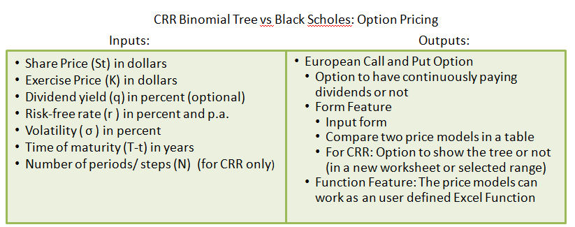
Friday, March 15, 2013

Userforms and Algorithm for Indiv Project

In class, we are to make an outline. As to how is our project supposed to work. Since I've done the logistics of the code for CRR tree and BS, I will continue on how am I supposed to ask data from the user and how am I supposed to show my output. The following slides are supposed to be my guideline for that. This is supposed to be a scratch userform

The picture below also show my initial input-output plan, and the proposed plan. I included this for the intention of not becoming lost along the way.
The initial plan:


The proposed plan


Thursday, March 14, 2013

VBA: OLS and SSE

This is a part of our class exercise. Also can be seen in the OLS and SSE excel file. The problem involved:
  •  Getting the results of the regression and find the regression estimate per row and compare with the actual, 
  • Computing for the error and the squared error
  • Displaying the results of regression and the sum of errors in a new worksheet
  • Creating a form for that,
  • And running the regression program dynamically
I reused and revised the code in the post Autoregression in functions, in particular the  Function OLS() to regress. In addition, I made up a form getting the data dynamically. Although test for errors were not included.

Functions and Subs
  • xM(x1) - Function that creates the x matrix
  • CommandButton1_Click() -serves as the test button or the Ok button. or also known as my input - output button because it determines what is your input and creates the output.
  • CommandButton2_Click() - the cancel button
  • OLS(y, x) - the revised OLS function. Its output are the betas
  • SSE(y, x) - solves for the SSE of the regressed y,x
Learning

I spent almost half of the class figuring out why the error mmult property cant run keeps popping up. and after a few hours I found out where I got it wrong. The logic of the code is correct but the parameters of the inputs are wrong. So lesson of the day is: Kung tama ang logic, at mali naman sa pinag gamitan. Mali pa rin yun. It works in real life.

The Form

Simple right :)

The Code


Private Sub CommandButton1_Click()
    y = Range(RefEdit1.Text)
    x1 = Range(RefEdit2.Text)
    
    'creating x matrix
    x = xM(x1)
    
    'regress
    param = OLS(y, x)
    
    'output Sheet
    Sheets.Add
    Range("A1") = "Solution Matrix"
    Range("A" & 2) = "Constant"
    For i = 2 To UBound(param)
        Range("A" & 1 + i) = "x" & i - 1
    Next i
    Range("B2").Select
    ActiveCell.Range(Cells(1, 1), Cells(UBound(param), 1)) = param
    Range("D1") = "Sum of Squared Errors"
    Range("D2") = SSE(y, x)
    
    Unload Me
End Sub

Private Sub CommandButton2_Click()
    Unload Me
End Sub

Private Function xM(x1)
    'adding ones to for coefficients in x matrix
    x = Range(Cells(1, 1), Cells(UBound(x1), UBound(x1, 2) + 1))
    For j = 1 To UBound(x, 2)
        For i = 1 To UBound(x)
            If j = 1 Then
                x(i, j) = 1
            Else
                x(i, j) = x1(i, j - 1)
            End If
        Next i
    Next j
    
    xM = x
End Function
    
Private Function OLS(y, x)
 'regression, getting betas and coefficient
 'given the matrix y and x
    
    xtrans = Application.WorksheetFunction.Transpose(x)
    xtx = Application.WorksheetFunction.MMult(xtrans, x)
    xtxinv = Application.WorksheetFunction.MInverse(xtx)
    xtxinvxt = Application.WorksheetFunction.MMult(xtxinv, xtrans)
    bsol = Application.WorksheetFunction.MMult(xtxinvxt, y)
    OLS = bsol
    
End Function

Private Function SSE(y, x)
    'sum of squared errors
    
    param = OLS(y, x)
    
    model = Application.WorksheetFunction.MMult(x, param)
    
    SumErrors = 0
    For i = 1 To UBound(x)
        SumErrors = SumErrors + (y(i, 1) - model(i, 1)) ^ 2
    Next i
    
    SSE = SumErrors
End Function

Saturday, March 9, 2013

Interest Rate Models

The class groups discussed two of term structure models: The Vacisek Model and the CIR term model.  These models are used to model interest rates.

What about the models:

  • equilibrium type of model
  • uses the Mean Reversion 
  • offer benefits since they are numerically quite simple and easy to solve with computers
  • very helpful in finding the important factors. 
  • interesting and widely tested empirically since they offer closed form solutions of their conditional and steady state density functions.
  • possible to get negative interest rates
Given the following:
  • $\Delta t = T-t$ 
  • $a$ as the speed of mean reversion
  • $\mu$ as the long run average rate
  • $r$ as the current state
  • $\sigma$ as the volatility
We can get the models:


CIR Model:
\[ P(t,T) = A(T-t)e^{-B(T-t)r}\]
where: \[ A(T-t) = \left [   \frac{2 \gamma e^{(a+ \gamma)(T-t)/2}} {(\gamma +a)(e^{\gamma (T-t)}-1} \right ]^{2ab/ \sigma^2} \]
and
\[ B(T-t) = \frac {2(e^{\gamma (T-t)}-1)}{(\gamma+ a)(e^{\gamma (T-t)}-1)+2 \gamma}\]


Vacisek Model:
\[ P(t,T) = A(T-t)e^{-B(T-t)r}\]

where: \[ A(T-t) = \text{exp} \left [ \frac{ ( B(T-t) - T+t ) (a^2b-\sigma^2/2)}{a^2} -\frac{\sigma^2 B(T-t)^2}{4a}\right ] \]
and
\[ B(T-t) = \frac {1-e^{-a(T-t)}}{a}\]

Comparing these two models, they have the same process only that the parameters $ A(T-t)$ and  $B(T-t)$ are different.


Sources: 

  • Hull book
  • Groups ppt. They simplified the process.

Friday, March 8, 2013

Monte Carlo: Antithetic and QuasiRandom

Please see: "Antithetic and QuasiRandom.xls"

As I have came to understand, the Antithetic and QuasiRandom is used to reduce the variances.

Antithetic technique:

  • Each time random variable r is drawn, its complement 1-r calculated and used to drive a parallel run of the simulation. This tends to lead to negatively correlated output values; hence lower variance
  • Example: this is from Monte Carlo - Antithetic and Quasi-Random.xls and it's quite direct to the point.
    • Table: The rand generates the random variable, and the randns generate the distribution. S1 solves $S_T$ of the simulation. S2 solves for antithesis of $S_T$ of the simulation. Then we get the payoffs for each S1 and S2. Then get the average payoff. Then we do it many many times. 
    • MC Value: Get the average of the avg pay and discount it to get the present value of the option. 

QuasiRandom technique:

  • We use Low Discrepancy Sequences to determine the random variables
    • Faure Sequence
    • Halton Sequence
    • Sobol Sequence
  • Inverse normal distribution
    • Box-Muller transform
  • Example: This is from Monte Carlo - Antithetic and Quasi-Random.xls 
    • Table: it uses Faure Sequence to determine the random variable, then Box-Miller transformation is used to determine the inverse normal distribution. Then we get $S_T$ for the share price and get the payoff.
    • MC Value: Get the average of the payoff and discount it to get the present value of the option. 

As can be seen in the graph below, Monte Carlo simulation, both Quasi and Antithetic Variate, converges to Black Scholes formula.


Source: Monte Carlo - Antithetic and Quasi-Random.xls 

Monte Carlo Option Pricing

Our group reported on Monte Carlo Option Pricing:


Notes:


Monte Carlo
  • important is how to generate the random distribution.
  • Do not rely on this as a black box solution..
  • We can look at the historical data.
  • We can do this as a project – straight forward models from hull or wilmott to generate the price setting model..to value our payoff.

Slide 3 - The Entire slides focused on Option Pricing. But for Portfolio Statistics we have 3 important concepts:
  • Find an algorithm for how the most basic investments evolve randomly. 
    • Equities: 
      • often the lognormal random walk
      • can be represented on a spreadsheet or in code as how a stock price changes from one period to the next by adding on a random return. 
    • Fixed-income
      • BGM model in modeling how interest rates of various maturities evolve
    • Credit 
      • A model that models the random bankruptcy of a company. 
      • Can represent any interrelationships between investments  which can achieved through correlations.
  • Understand the derivatives theory for after performing simulations of the basic investments, there is a need to have models for more complicated contracts that depend on them such as options/derivatives/contingent claims. 
  • May be able to use the results in the simulation of thousands future scenarios to examine portfolio statistics 
    • Ie. how classical Value at Risk can be estimated
Slide 4

Risk-neutrality assumption – We make the assumption that investors are risk neutral, i.e., investors do not increase the expected return they require from an investment to compensate for increased risk.

Cox and Ross (1976) have shown that the assumption of risk neutrality can be used to obtain solutions of option valuation problems.’ This implies that the expected return on the underlying asset is the risk-free rate and that the discount rate used for the expected payoff on an option  is the risk-free rate.


Slide 6 - Stages from Watsham book and the original Boyle paper

Slide 7 - 14 - Option pricing_monte carlo example.xls


Slide 15 -Example from Wilmott: 

Its difference from watsham is that the watsham example creates random variables with empirical data's probability distribution. Wilmotts random variables are with uniform probability distribution.

***Note: have to understand the "Antithetic and QuasiRandom.xls"


VBA: CRR European, BS, and American Options

How the code works:

This is what I have done so far. It contains the basic codes for BS Merton, CRR European and American Options. It also includes the greeks, delta, gamma and theta. I coded it the way I understood options. In a visual way. Though it's not yet tested for other numbers.

Sub Test() just contains the input and output of what is happening on the code since I'm just halfway done. The "user" part and the "output" part isn't completed yet. It is just presentable.

GenEurAm() contains the code in solving the option value and generating the values involved in the tree for Amerucan and European options.

Greeks() computes for the greeks and has an output table of the greeks.

GenBS() is the Black-scholes Merton way for computing european options

DrawTree() generates a designed tree complete with asset price and option prices. Though it is not as efficient as I would like. I computed for 100 steps and it took 9 secs to generate the tree alone.

DrawTree2() generates a tree in a more efficient manner. I have a choice whether what tree to generate. Either the price tree or the option value tree.

The functions are just a way to make the code flexible and more user-friendly. Though I don't know what to do with them right now at my codes..maybe later it will be handy.

Will do the user part next. and then the output sheets.

New to the code:
  • Learned: Declaring variables outside the sub or function
  • ActiveCell.Offset(0, 0).Value 
  • Range(starter).Offset(0, 0).Value
  • On properties of the range
    • With ... End With 
    • .Interior.ColorIndex = 34
    • .Borders.Weight = xlThin
    • .HorizontalAlignment = xlCenter
    • .Value = OptionValue(lp, j)
Code:

Public OptionValue() As Double

Public Price() As Double
Public bsOV As Double

Public kind As String
Public z As Integer

Public So As Double
Public K As Double
Public q As Double
Public r As Double
Public T As Double
Public n As Integer

Sub Test()
    
    So = 100
    K = 95
    q = 0
    r = 0.08
    vol = 0.3
    T = 0.5
    n = 5
    'kind = "a" 'american = a, european = e
    z = -1 'for call z= -1, if for put z= -1
    
    starter = "C11"
    
    Range(starter).Offset(0, 0).Value = "European:BS"
    Range(starter).Offset(0, 1).Value = GenBS(z, So, K, q, r, vol, T, n)
    
    Call GenEurAm("e", z, So, K, q, r, vol, T, n)
    Range(starter).Offset(1, 0).Value = "European:CRR"
    Range(starter).Offset(1, 1).Value = OptionValue(0, 0)
    
    Range(starter).Offset(3, 0).Value = "Asset Prices:"
    Range(starter).Offset(4, 1).Select
    Call DrawTree2(n, Price)
    Range(starter).Offset(n + 5, 0) = "European Option Prices:"
    Range(starter).Offset(n + 6, 1).Select
    Call DrawTree2(n, OptionValue)
    
    Call GenEurAm("a", z, So, K, q, r, vol, T, n)
    Range(starter).Offset(1, 3).Value = "American:CRR"
    Range(starter).Offset(1, 4).Value = OptionValue(0, 0)
    Range(starter).Offset(2 * n + 7, 0) = "American Option Prices:"
    Range(starter).Offset(2 * n + 8, 1).Select
    Call DrawTree2(n, OptionValue)
    
    Range(starter).Offset(3 * n + 9, 0).Value = "Greeks:"
    Range(starter).Offset(3 * n + 10, 1).Select
    Call Greeks
    
End Sub

Private Sub GenEurAm(kind, z, So, K, q, r, vol, T, n)
    
    'computation of the formulas
    u = Exp(vol * Sqr(T / n))
    d = 1 / u
    b = Exp((r - q) * T / n)
    p = (b - d) / (u - d)
    df = Exp(r * T / n)
    
    'Price tree
    ReDim Price(0 To n, 0 To n)
    
    'American and European Option tree
    ReDim OptionValue(0 To n, 0 To n)
    
    For j = n To 0 Step -1
        For lp = 0 To j
            
            'Price tree
            Price(lp, j) = So * u ^ lp * d ^ (j - lp)
            whenX = z * (Price(lp, j) - K)
            
            'option tree
            'at the end nodes
            If j = n Then
                OptionValue(lp, j) = Application.WorksheetFunction.Max(whenX, 0)
            'at other nodes
            Else
                whenNotX = (p * OptionValue(lp + 1, j + 1) + (1 - p) * OptionValue(lp, j + 1)) / df
                'for american option
                If kind = "a" Then
                    OptionValue(lp, j) = Application.WorksheetFunction.Max(whenX, whenNotX)
                'for european option
                ElseIf kind = "e" Then
                    OptionValue(lp, j) = whenNotX
                End If
            End If
        Next lp
    Next j

End Sub

Private Sub Greeks()
    'after calculating the prices and the option values
    'brute force
    
    Dim del(0 To 2) As Double
    Dim gam As Double
    Dim the As Double
        
    del(0) = (OptionValue(0, 1) - OptionValue(1, 1)) / (Price(0, 1) - Price(1, 1))
    
    del(1) = (OptionValue(0, 2) - OptionValue(1, 2)) / (Price(0, 2) - Price(1, 2))
    del(2) = (OptionValue(1, 2) - OptionValue(2, 2)) / (Price(1, 2) - Price(2, 2))
    gamma = (del(1) - del(2)) / (Price(0, 1) - Price(1, 1))
    
    theta = (OptionValue(1, 2) - OptionValue(0, 0)) / (2 * T / n)
    
    ActiveCell.Offset(0, 0).Value = "Delta"
    ActiveCell.Offset(0, 1).Value = del(0)
    ActiveCell.Offset(1, 0).Value = "Gamma"
    ActiveCell.Offset(1, 1).Value = gamma
    ActiveCell.Offset(2, 0).Value = "Theta"
    ActiveCell.Offset(2, 1).Value = theta
    
End Sub

Private Function GenBS(z, So, K, q, r, vol, T, n)
    'Black Scholes Merton
    
    'defining the parts
    d1 = Application.WorksheetFunction.Ln(So / K) + (r - q + vol ^ 2 / 2) * T / (vol * Sqr(T))
    d2 = Application.WorksheetFunction.Ln(So / K) + (r - q - vol ^ 2 / 2) * T / (vol * Sqr(T))
    
    If z = 1 Then
        nd1 = Application.WorksheetFunction.NormSDist(d1)
        nd2 = Application.WorksheetFunction.NormSDist(d2)
    ElseIf z = -1 Then
        nd1 = Application.WorksheetFunction.NormSDist(-d1)
        nd2 = Application.WorksheetFunction.NormSDist(-d2)
    End If
    
    'getting black scholes
    GenBS = z * (So * Exp(-q * T) * nd1 - K * Exp(-r * T) * nd2)
    
End Function

Private Sub DrawTree(n, starter)
    'with design, not efficient
    
    r = 2 * (2 * n + 1)
    For j = 0 To n
        nrow = r / 2 - 2 * j
        For lp = j To 0 Step -1
            With Range(starter).Offset(nrow, j)
                .Interior.ColorIndex = 42
                .Borders.Weight = xlThin
                .HorizontalAlignment = xlCenter
                .Value = Price(lp, j)
            End With
            With Range(starter).Offset(nrow + 1, j)
                .Interior.ColorIndex = 34
                .Borders.Weight = xlThin
                .HorizontalAlignment = xlCenter
                .Value = OptionValue(lp, j)
            End With
            nrow = nrow + 4
        Next lp
    Next j
End Sub

Private Sub DrawTree2(n, ranger)
    'after calculating for the prices and the optionvalue
    'simple lng
    
    For col = n To 0 Step -1
        For nrow = n - col To n
            ActiveCell.Offset(nrow, col).Value = ranger(n - nrow, col)
        Next nrow
    Next col
    
End Sub

Public Function EuroCall(So, K, q, r, vol, T, n)
    Call GenEurAm("e", "1", So, K, q, r, vol, T, n)
    EuroCall = OptionValue(0, 0)
End Function

Public Function EuroPut(So, K, q, r, vol, T, n)
    Call GenEurAm("e", "-1", So, K, q, r, vol, T, n)
    EuroPut = OptionValue(0, 0)
End Function

Public Function AmCall(So, K, q, r, vol, T, n)
    Call GenEurAm("a", "1", So, K, q, r, vol, T, n)
    AmCall = OptionValue(0, 0)
End Function

Public Function AmPut(So, K, q, r, vol, T, n)
    Call GenEurAm("a", "-1", So, K, q, r, vol, T, n)
    AmPut = OptionValue(0, 0)
End Function

Public Function BSCall(So, K, q, r, vol, T, n)
    BSCall = GenBS("1", So, K, q, r, vol, T, n)
End Function

Public Function BSPut(So, K, q, r, vol, T, n)
    BSPut = GenBS("-1", So, K, q, r, vol, T, n)
End Function

Sources:


http://www.cpearson.com/excel/classes.aspx

http://dmcritchie.mvps.org/excel/colors.htm

http://www.global-derivatives.com/index.php/component/content/52?task=view

Black, F. & Scholes, M. "The Pricing of Options & Corporate Liabilities" The Journal of Political Economy (May '73)

Hull, J. "Options, Futures & Other Derivatives" 5th Edition 2002 - Chapter 12

Merton, R. "Theory of Rational Option Pricing" Bell Journal of Economics & Management (June '73)


Mathlab Example, European or American options
          - http://www.goddardconsulting.ca/matlab-binomial-crr.html

American Call Option, Greeks, Python, getting data from google finance, etc., Concepts and formulas included
          - http://www.quantandfinancial.com/2012/11/cox-ross-rubinstein-option-pricing-model.html

Option Pricing Formulas book, Complete with greeks and American Options p279-288
          - http://r2-d2.bu.edu/AT__The_Complete_Guide_to_Option_Pricing_Formulas__2nd_ed_.pdf

Option Calculator
         - http://www.volatilitytrading.net/cox_ross_rubenstein_calculator.htm


VBA: Bond Valuation II

In our class discussion, the prof taught me a different way of coding using the record macro and worksheets.

  • Made me think it will be helpful in creating excel sheet forms and output data.
  • Discovered ActiveCell.Offset(r,c)

Here's the code:


Sub Macro3()

For i = 1 To 108

Application.ScreenUpdating = False

Sheets("DATA Process").Select
Range("A1").Select

'dito ka lng nagloop and it works for all
ActiveCell.Offset(i, 0).Range("A1:E1").Select
Selection.Copy

Sheets("Scratch").Select
Range("A2").Select
Selection.PasteSpecial Paste:=xlPasteValues, Operation:=xlNone, SkipBlanks _
        :=False, Transpose:=False

Range("F15").Select
Selection.Copy

Sheets("DATA Process").Select
ActiveCell.Offset(0, 6).Range("A1").Select
Selection.PasteSpecial Paste:=xlPasteValues, Operation:=xlNone, SkipBlanks _
        :=False, Transpose:=False

Next i

End Sub

Saturday, March 2, 2013

CRR: Option Pricing

This post dwells on CRR tree with the application of Option Pricing.

I admit the first method is the simpler one but only used for European Option Pricing. However if I wanted to generalize European and American Option Pricing, it is better explained in the second method.

Inputs:
  • Share Price (S) in dollars
  • Exercise Price (K) in dollars
  • Dividend yield (q) in percent (continuously paying)
  • Risk-free rate (r ) in percent and p.a.
  • Volatility ( σ ) in percent
  • Time of maturity (T) in years
  • Number of periods/ steps (n)  
Output: European Call and Put Option

Method 1: Direct Approach (similar to Haug book and  Jackson and Staunton book)

First we get the necessary $u$, $d$ and $p$ by using the following formulas:

  • $u = e^{\sigma \Delta{t}}$
  • $d = e^{-\sigma \Delta{t}}$  or simply $d = \frac{1}{u}$
  • $p = \frac{ e^{(r-q)\Delta{t}} - d }{u-d} $

where $\Delta{t} = \frac{T}{n}$.


European Options are only exercised at the end of the period. That means we are just looking at the end nodes of the tree. In this case, we solve for the probability at each of the end nodes, multiply it by each payoff, sum it up and then get its present value. The formula for call and put option are as follows:

\[ c= e^{-rT} \sum_{i=0}^{n}  {_n}C_{i}  p^i  (1-p)^{n-i} \text{max}[Su^i d^{n-i} - K, 0] \]
\[ p= e^{-rT} \sum_{i=0}^{n}  {_n}C_{i}  p^i  (1-p)^{n-i} \text{max}[K-Su^i d^{n-i}, 0] \]
where
  • $e^{-rT}$ is the discounting factor
  • ${_n}C_{i}  p^i  (1-p)^{n-i}$ is the probabilities at each final node $n$ at step $i$
  • $Su^i d^{n-i}$ is the prices at each final node $n$ at step $i$
  • $\text{max}[Su^i d^{n-i} - K, 0]$ is the payoff for call option.
  • $\text{max}[K-Su^i d^{n-i}, 0]$ is the payoff for put option.
Notice that the only difference for put and call options are their payoffs.
Example: same as in Haug approach sheet in CRRforProj.xlsm 

Given the following values, we want to compute for the European Call and Put Option.


Solution:


Method 2: Using Trees (also similar to Haug book, Jackson and Staunton book and the presentation found in earlier post.)


First we get the necessary $u$, $d$ and $p$ by using the following formulas:

  • $u = e^{\sigma \Delta{t}}$
  • $d = e^{-\sigma \Delta{t}}$  or simply $d = \frac{1}{u}$
  • $p = \frac{ e^{(r-q)\Delta{t}} - d }{u-d} $
where $\Delta{t} = \frac{T}{n}$.


Then we create the tree for price. The formula is  $Su^i d^{n-i}$ at each node $j$ at step $i$.

Then we create the tree for the option price. The end nodes, we compute for the payoff. It is the same whether it is European or American options.

  • $\text{max}[Su^i d^{n-i} - K, 0]$ is the payoff for call option.
  • $\text{max}[K-Su^i d^{n-i}, 0]$ is the payoff for put option.

At the remaining nodes, European and American Option Prices differ even if the process is the same. It is because European option only exercises the end of the period while American options can be exercised earlier. So the formula for the remaining nodes $j$ at step {i} are as follows:

  • European Call and Put: $O_{i,j}= e^{-r \Delta{t}} (p O_{i+1,j+1}+(1-p)O_{i,j+1} ) $
  • American Call: $OV_{i,j} = \text{max}[Su^i d^{n-i} - K, e^{-r \Delta{t}} (pO_{i+1,j+1}+(1-p)O_{i,j+1} )]$
  • American Put: $OV_{i,j} = \text{max}[K-Su^i d^{n-i},e^{-r \Delta{t}} (pO_{i+1,j+1}+(1-p)O_{i,j+1} )]$
Example:

for European Option Example: please see earlier post.

For American Option Example: same as in American Tree sheet in CRRforProj.xlsm 


Given the following values, we want to get the American Put Option Price.


Solution:


Source: 

  • http://r2-d2.bu.edu/AT__The_Complete_Guide_to_Option_Pricing_Formulas__2nd_ed_.pdf
  • Advance Modelling in Finance using Excel and VBA by Jackson and Staunton

Friday, March 1, 2013

Black Scholes: Option Pricing

I thank God for blogging. It forces me to put my thoughts into words, helping me to think clearly.

Inputs:
  • Share Price (S) in dollars
  • Exercise Price (K) in dollars
  • Dividend yield (q) in percent (continuously paying)
  • Risk-free rate (r ) in percent and p.a.
  • Volatility ( vol ) in percent
  • Time of maturity (T) in years or Option Life (T-t) (it doesnt matter
Output:
  • European Call and Put Option
Method: Black-Scholes Merton
  • With or without dividends, we can use the same formula.
    • d1 = Ln(So / K) + (r - q + vol ^ 2 / 2) * T / (vol * Sqr(T)
    • d2 = Ln(So / K) + (r - q - vol ^ 2 / 2) * T / (vol * Sqr(T))
    • z  * (So * Exp(-q * T) * nd1 - K * Exp(-r * T) * nd2)
      • if z = 1, we have a call option 
      • if z = -1, we have a put option
      • nd1 and nd2 are standard normal distribution of d1 and d2 respectively.
Sources:
  • http://www.global-derivatives.com/index.php/component/content/52?task=view
  • Black, F. & Scholes, M. "The Pricing of Options & Corporate Liabilities" The Journal of Political Economy (May '73)
  • Hull, J. "Options, Futures & Other Derivatives" 5th Edition 2002 - Chapter 12

VBA: Bond Valuation as Function

Given:  Data from automation macro Data.xls

On that excel sheet, we are given: term, credit rating, coupon rate and par value. Compute for the PV Cash flow/Market Value of the bond of the using the spot yield curve with the credit rating add on.

How the code works:

The Market Value is solved using the user defined function MV(term, creditrate, coupon, pvalue) with dynamic spot yield and credit rating, by letting the user define such.

1. We define the discounting factor depending on the requirements by using Lookup() of Excel.
2. We then use the discount factor in getting the cash flows. We sum up the PV of every year for the results. 

The AutoCompute() Sub automatically computes for the MV given number n of records.

New to the code:
  • Defining Dimensions
  • Application.WorksheetFunction.Lookup(i, spotYC)
  • r = Range("A2").End(xlDown).Row - 1
Other learnings:
  • one dimensional array: http://www.vbtutor.net/VBA/vba_chp21.htm
  • Dim rate(10) as double
Code:

Function MV(term As Integer, CreditRate As String, Coupon As Double, pv As Double)
    
    Dim sumMV As Double
    Dim drate As Double
    Dim s As String
    Dim a As String
    
    s = Range("o6") 'range of spotyield
    spotYC = Range(s)
    a = Range("o7") 'range of credit rating addon
    CreditReq = Range(a)
    
    'determining individual credit rate Add on
    
    addon = Application.WorksheetFunction.Lookup(CreditRate, CreditReq)
    
    'determining cashflows
    
    sumMV = 0 'summing cashflows along each term
    For i = 1 To term
        srate = Application.WorksheetFunction.Lookup(i, spotYC) 'determine the spot yield rate per year
        drate = srate + addon
        sumMV = (Coupon * pv) / (1 + drate) ^ i + sumMV 'for cashflows with coup*pv
    Next i
    sumMV = sumMV + pv / (1 + drate) ^ term 'for the last cashflow


    If term = 0 Then
        sumMV = 0
    End If

    'throwing back to excel
    MV = sumMV

End Function


Sub AutoCompute()
    
    Dim term As Integer, CreditRate As String, Coupon As Double, pv As Double
    
    'first row serves as Titles so start with
    r = Range("A2").End(xlDown).Row - 1
      
    For i = 1 To r
        term = Range("b" & 1 + i)
        CreditRate = Range("c" & 1 + i)
        Coupon = Range("d" & 1 + i)
        pv = Range("e" & 1 + i)
        Range("f" & 1 + i) = MV(term, CreditRate, Coupon, pv)
    Next i
    
End Sub